This document describes a workflow for drone mapping and object counting/location using open-source software. The specific tools involved are: WebODM (OpenDroneMap), YOLOv7/PyTorch, QGIS with Deepness plugin, and some custom scripts written to simplify various steps in the process.
This workflow is based on a process developed and used by Twomile, with input from aerial mapping and conservation experts in a variety of organizations. (See “Credits” further down the page.)
Benefits of an open-source workflow include:
-
All data can be processed 100% locally
No need for cloud storage or hosting. Processing supported on mid-grade off-the-shelf hardware and operating systems.
-
Chain of custody
Maintain control of sensitive data. Training and analysis data need not be shared with any third party.
-
Transparency
Open source software can be reviewed. All processing steps are available for examination.
-
Low cost (or no cost)
No software purchase required. No ongoing subscriptions or fees required.
Please note: The accuracy of the detection and counting is highly dependent on how well-trained your software model is. Training and accuracy of computer vision models is a huge field and is not addressed here.
You are encouraged to use this workflow as a reference in your own organization. We appreciate any feedback on the process and documentation (see “Feedback and Collaboration” section, below). You can also download a PDF of this page.
This workflow is described in five main areas:
- Preparation and Data Collection
- Processing Aerial Photos
- Training an Object Detection Model
- Counting and Locating Objects
- Verification and Refinement
 Main areas of the open source object counting and location workflow
1 - Preparation and Data Collection
The first area of the workflow is primarily planning and setup. It also involves the collection of aerial data for your project.
1.a - Identify Project Goals
Knowing the end goal(s) of your project will save you time and headaches. Teaching a computer to detect and count objects requires you to know what you’re counting, and in what environment(s) so that you can gather or create the appropriate training data. Also, you should understand the desired resolution for your aerial data. e.g., how many cm/pixel, and what level of accuracy is “good enough” for your automated counts.
1.b - Identify Processing Hardware, Confirm System Requirements
This workflow targets a medium-grade PC with the following specifications:
- 32+ GB RAM
- 500+ GB Hard Drive
- Windows 10 or Ubuntu 20+ with Docker
Most mid-tier gaming laptops from 2021 or later should be sufficient for this. Having a dedicated GPU is helpful but not required. Because some of the processing tasks are resource-intensive and need to run for many hours, you will probably find it useful to set this up on a dedicated processing machine. Twomile uses two older rebuilt desktops from Dell and HP with these specs: i7 CPU, 64-128 GB RAM, 2 TB HDD.
1.c - Software Setup
You will need to install the following software applications. All are open source. You can install everything on a single PC, but you can also separate them if preferred.
Python 3 and PIP
You may already have them, but follow the instructions here if not. Python 3 is required (not 2).
WebODM (OpenDroneMap)
For Windows, the Windows Installer is the easiest. It costs about $60 and you own it forever. You can also install on Windows or Linux so that it uses Docker. The Docker approach is 100% free and it is also very easy, if you are familiar with Docker.
Some Linux distributions support a native installation also, but there are many steps. If you are comfortable installing Linux applications that way, it could be a good approach for you.
After installing WebODM, start the application and create a user login when prompted.
YOLOv7
Clone the YOLOv7 repo. Edit requirements.txt to uncomment these three libraries in the Export section: onnx, onnx-simplifier, scikit-learn. Then, use PIP to install the YOLO dependencies:
cd yolov7
pip install -r requirements.txt
Also, download the pretrained yolov7 file yolov7_training.pt for use in your training. Put this file in the root of your yolov7 directory.
QGIS
Follow their instructions to download and install the latest. This workflow was developed using QGIS 3.28, but most recent versions should work fine.
QGIS is a large and complex GIS application. If you are familiar with other GIS software (e.g., ArcGIS) you should be able to find your way around, but you might want to consult some getting started tutorials if you are not already familiar with QGIS.
Deepness Plugin
Use the QGIS plugin manager to install the plugin. It requires some additional python libraries be installed, to support the plugin. When you run the plugin for the first time, it should walk you through the steps to install the additional python libraries. If that doesn’t work for some reason, consult the Deepness docs and review the installation instructions to try manually installing the additional items.
If the Deepness plugin is installed and working correctly, you will see this icon in the QGIS toolbar.
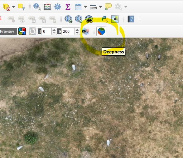 View of Deepness plugin icon in QGIS toolbar
Twomile Scripts
Clone the Twomile yolo-tools repo. These are scripts to help with various stages of the workflow. It is helpful to have the yolo-tools directory at the same level as your yolov7 directory.
1.d - Gather Aerial Data to be Processed
Twomile collects aerial data using DJI Phantom 4 Pro drones, with flight planning and execution handled by the Pix4D Capture, DroneDeploy, or MapsMadeEasy iPad apps.
We have not identified open source tools for flight planning and data collection using DJI equipment, so this section contains no specific recommendations. Gather your aerial photos via your existing approach.
2 - Processing Aerial Photos (OpenDroneMap/WebODM)
2.a - Test Run
Open WebODM and create a new processing task using a small sample of your aerial data. A good start is about 50 photos in the same general area (e.g., the first 50 photos in the set, or the last 50). Leave the task configuration options on their defaults. Run the task. It should complete in less than 30 minutes, and you should be able to see a small portion of your subject area in both 2D and 3D view. If the task fails, you will need to do some troubleshooting. Get this working before moving on to the next step.
2.b - Process Aerial Photos
Processing aerial photos into 2D and 3D geospatial data is a big topic, with many configuration options. If you are using common drone hardware (e.g., DJI, Skydio, Autel), the default options are probably fine to start. Consult the ODM documentation and forums for help with various configuration and processing options appropriate to your specific subject. When you are satisfied with your orthophoto, proceed to the next step.
2.c - Export Orthophoto
From the WebODM task list, export the Orthophoto of your subject area. Use the default projection and format. This will download a TIF file of your subject area that is georeferenced. Depending on the number of aerial photos used, this may be a pretty large file (hundreds of MB). This is the file that will be examined for object detection and counting.
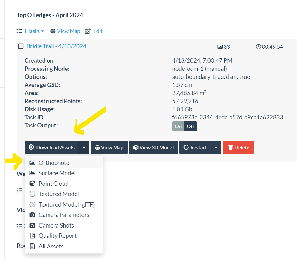 Downloading an orthophoto from WebODM
3 - Training an Object Detection Model (YOLOv7/PyTorch, Scripts)
The accuracy of your object detection and counts data is mainly a function of how good your model is. However, computer vision and object detection are a massive topic and most details will not be covered here. The purpose of this workflow is to help string together the process of using some model to perform counts on your aerial data. This workflow will get you up and running, but you will certainly need to invest additional time and energy developing a mature understanding of computer vision model development, so you can get the best possible results from your aerial data.
Note: After you have been through this entire workflow the first time, you will probably want to refine and improve your object detection model. If so, you will repeat these steps in Section 3. If you are satisfied with your model and you just want to run the model against new aerial data, you can skip Section 3. You don’t have to train a new model for every object detection/counting task. If you are looking for the same things in similar contexts, your model can be used over and over again.
3.a - Locate Relevant Training Data
You need to locate some aerial-view training data that can be used to train your model. If you want to detect birds, you need a bunch of photos of birds which have already been annotated with bounding box locations.
Some datasets are available on Kaggle. Some research projects also make their training data available. Try searching online for “annotated aerial photos” and your subject area - e.g., “annotated aerial photos +birds” to locate relevant publications and datasets. In developing this workflow, we used some of the training data made available by Weinstein et al (2022).
The annotations may be in a different data format, and may need to be converted. The Twomile yolo-tools repo contains two conversion scripts. convert-pascal.py is useful for converting PASCAL VOS format annotation files (XML) into the format expected by YOLOv5/v7. The script convert-weinstein.py can be used to convert annotation data provided with the Weinstein et al (2022) training datasets. If you intend to use either script, you should review the code and ensure it is applicable to your annotation data. You may need to adjust the scripts or create new scripts based on these. After converting, use test-converted.py to visually check a random sample of your converted annotation data overlaid on its image file.
If you cannot find suitable training data, you will need to create your own. Read up on training data labeling and install a tool such as BBoxEE or LabelImg. There are many.
Finally, you need to divide your images into a training set, a validation set, and a test set. Use the Twomile script partition.py to create these in the appropriate directories.
Note: Several of the scripts mentioned in this section are heavily based on code provided in this excellent article on the Paperspace blog.
3.b - Test Run
Computer vision model training is resource-intensive and takes a long time (many hours). When you have your training data together, start with a quick test run of the model training. It won’t produce a good model, but it will tell you whether everything is working.
For your test run, you want to use all your data (all photos/annotations) but you only want to train for a short time (3 cycles, or “epochs”). Copy your partitioned data into the YOLO data directory:
cp yolo-tools/out/partition yolov7/data/test1
cp yolo-tools/cfg/yolo-data.yaml yolov7/data/test1.yaml
Then, edit test1.yaml and set the appropriate number of classes and class names for your training data. The file paths should already be correct.
Next, edit the Twomile script train.sh and set NUM_EPOCHS to 3 if it is not already set to that value. Set the IMG_SIZE parameter to something close to the max width or height (whichever is larger) of your training images. YOLO wants this number to be a multiple of 32, so if your images are 900px you should enter 928. YOLO should also make the adjustment for you automatically if you just enter the exact size of the images.
Set RUN_NAME to test1_3ep_det or something that will make sense to you. This sets the name of the output directory for the YOLO training run.
Finally, go to the yolo7 directory and run the train.sh script from there (note the paths):
cd yolov7
../yolo-tools/train.sh
This will start the training process. It will take a few minutes per epoch, but this process will tell you pretty quickly if things aren’t working. If the process doesn’t complete successfully or you see python errors, you need to troubleshoot and resolve your issues before running the real thing in the next step.
3.c - Train Model
If your test run completed successfully, you are ready to fully train your model. Look at the console output and make a note of the time required to complete 3 epochs. Multiply that time by 33, that that’s a reasonable estimate of how long the full training will take. (e.g., 30 minutes for 3 epochs means about 16.5 hours for 100 epochs).
Edit train.sh again and set NUM_EPOCHS to 100. Change the value of RUN_NAME to something meaningful for you (e.g., full_training_100ep_det). Run the training script again.
../yolo-tools/train.sh
This will start the full training. Your PC will be heavily burdened for several hours. You can expect the cooling fan to run most of the time. Make sure it can get plenty of airflow. Check the console output and ensure that the training has started correctly, and epochs are progressing.
Once complete, the files will be located in: yolov7/runs/train/[RUN_NAME]
You can make a few quick visual checks of files within this directory to see how well the model works against its test data.
- Look at the image “results.png” and check the graphs. The trend lines for Precision and Recall should become consistent and settle near a reasonably high value (e.g., 0.8). Box and Objectness should become more consistent. mAP values should become more consistent.
- Look at test_batch0_pred.jpg, test_batch1_pred.jpg, and test_batch2_pred.jpg. Objects should be detected and labeled correctly.
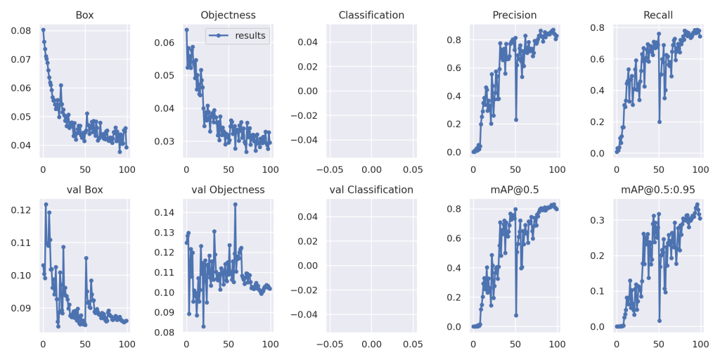 Example results.png image from YOLOv7 model training
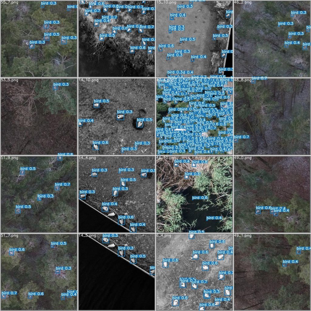 Example prediction output from YOLOv7 model training
3.d - Export to ONNX
You now have a usable YOLO object detection model. It could be used with the standard YOLO capabilities to detect objects in photos and videos. There’s a lot you can do already. However, for our purposes here we want to count and locate objects in our aerial data so we need to convert this model to ONNX format.
For this, we use the Twomile script export.sh. Edit that file and set RUN_NAME to match the value you set in train.sh (e.g., full_training_100ep_det). Set the value for IMG_SIZE to match the value you set in train.sh, also.
Stay in the yolov7 directory as we will run the script from there.
../yolo-tools/yolo/export.sh
This will create an ONNX version of the output in your model’s weights directory. e.g., full_training_100ep_det-yolo7-deepness.onnx Make a note of the filename and location, as you will need this for the next step.
3.e - Set Metadata
In addition to exporting the model to ONNX format, you will need to set some key parameters in the model configuration which allow it to be used by the Deepness plugin.
For this, we use the Twomile script metadata.py. To run the script, we pass in two parameters. The first is a path to the recently-created ONNX model, and the second is an output path for the updated model. (It creates a copy of the model, with appropriate metadata.)
Edit the metadata.py script and set your class names in the class_names variable. (This will be moved to a command-line argument eventually.)
Stay in the yolov7 directory as we will run the script from there.
python ../yolo-tools/metadata.py [INPUT_MODEL_PATH] [OUTPUT_PATH]
Check the script output and ensure the process has completed successfully. The script will show the path of the model with metadata. Make a note of this location, as you will need it when performing object counting in QGIS.
4 - Counting and Locating Object (QGIS/Deepness)
Once your model has been trained, exported, and adjusted successfully you can use QGIS with the Deepness plugin to detect, count, and locate objects in your subject area orthophoto. If you are working through everything the first time, it is a good idea to download a simple orthophoto and detection model to ensure that all the plumbing is correct in QGIS/Deepness.
4.a - Test Run
- Download this test orthophoto and this test detection model.
- Open QGIS and create a new project.
- Add the test orthophoto as a new raster layer.
- Confirm you have the Deepness plugin icon in the toolbar. Click it to open the Deepness configuration panel. Configure as below:
- Input layer: (the test orthophoto layer)
- Processed area mask: Entire layer
- Model type: Detector
- Model file path: (locate your file with metadata applied, from step 3.e)
- Resolution: 2.00
- Detector type: YOLO_v5_or_v7_default
- Confidence: 0.30
- IoU Threshold: 0.40
- (All other items can use the default values)
- Click ‘Run’
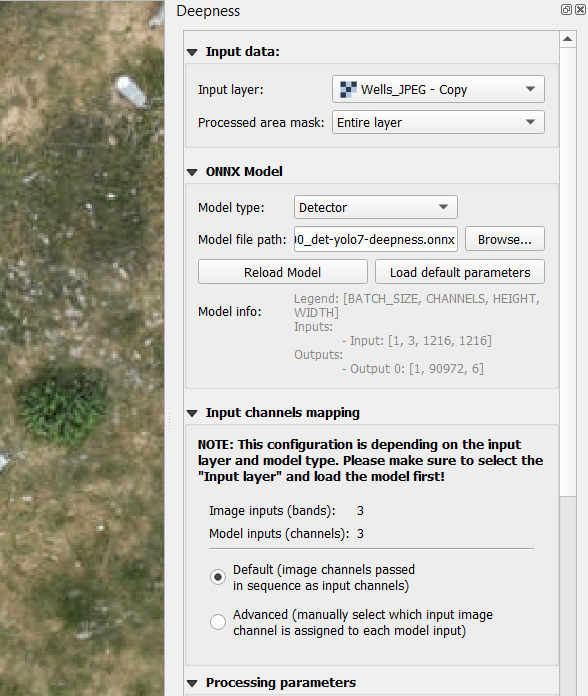 Deepness plugin parameters (top half)
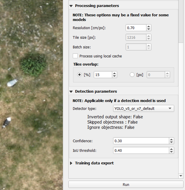 Deepness plugin parameters (bottom half) and Run button
You should see the progress bar in the middle of the bottom of the screen increasing from 0% to 100%. No errors should appear. At the end of the process, you should see a dialog showing “Detection done for 1 model output classes, with the following statistics: " (etc.) and an OK button. Click OK to continue.
If there were errors or the processing could not be completed, you will need to troubleshoot and resolve the error(s) before proceeding to the Count and Locate step.
4.b - Run Counting and Location
Once you have successfully run the test data, you’re ready to run counting and location on your own subject area.
- Create a new project in QGIS
- Add your aerial data orthophoto (see Step 2.c)
- Click the Deepness plugin icon (globe) and configure the plugin to use your trained model (see Step 3.e)
- Confirm the rest of the Deepness configuration settings match the test run (Step 4.a)
- Click ‘Run’
If there were errors or your processing was not completed, there is likely a problem with your ONNX object detection model. You will need to troubleshoot and resolve them.
If counting and location is successful, you will see the progress bar in the middle of the bottom of the screen increasing from 0% to 100%. No errors should appear. At the end of the process, you should see a dialog showing “Detection done for N model output classes, with the following statistics: (etc.) " and an OK button. Make a note of the total count shown in the dialog.
4.c - View Counts and Locations
Now you can view the locations of the detected objects. The Deepness plugin will create a new layer group called “model_output” with a vector layer containing rectangles (bounding boxes) for the located objects (e.g., “bird”).
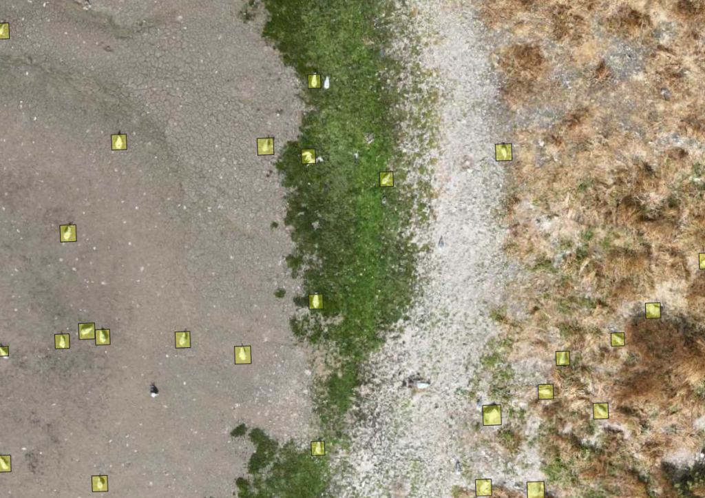 Birds detected and located in aerial data (orthophoto)
By this point, you have worked through all the complex technical plumbing to perform object detection, counting, and location. Congratulations! That’s no small accomplishment.
Probably, the results you see on-screen and in your count data are probably in the realm of “pretty good” or “okay”. You will probably need to spend time with configuration parameters and updating your object detection model training. There are several tips and resources in Step 5.b for refining your model. For now, we will continue with the mechanics of QGIS and using your data.
You may wish to rename the layer to something that gives you hints about the configuration or model used. e.g., change the layer group name to “Bird Counts” and change the layer itself to “Birds_Model1_200_03_04” to indicate that the layer shows the result of object detection model “Model1” at 2.00 Resolution, 0.3 Confidence and 0.4 IoU. You can also make all the usual GIS layer modifications like changing symbology and appearance, adding labels, etc.
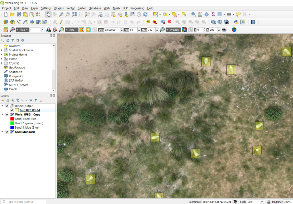 QGIS interface showing detected birds and associated layer information
To view the total count, right click the layer and select “open attribute table”. This opens the QGIS attribute table with a row for each detected object. There is no real data in the table other than feature ID (“fid”) but the table stats at the top of the window provide your count. e.g., “Features Total: 305, Filtered: 305, Selected: 0” indicates that 305 objects were detected in the orthophoto.
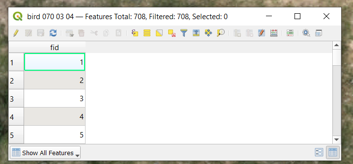 QGIS attribute table for detected features
Note: By default, your count/location layer is temporary so if you close QGIS or the project you will lose it. You should save the temporary layer by right clicking the layer, selecting “make permanent” and following the prompts to select a file format and location.
4.e - Export Counts and Locations
You may choose to perform all of your analysis within QGIS. It is a robust and capable tool. You may also wish to export your data for further analysis, archival, or sharing.
To export count and location data, right-click the data layer then “Export” and “Save Features As” and follow the prompts to select an appropriate file format and location.
 QGIS layer export dialog
5 - Verification and Refinement
5.a - Manual Checks
There are a variety of ways to check your counts. The easiest process is to methodically review the entire subject area in QGIS, noting objects that were missed by the model, or objects that were mistakenly identified and counted (false positive). You might just take manual notes about this, or you could create an additional layer to mark the locations of the errors. You can also use the very nice open source application DotDotGoose to perform a manual count and compare results with the model.
5.b - Refine Object Detection
Based on your verification results, you will likely wish to refine your object detection configuration and model. To get the best possible performance in counting and location, you need to train a really, really good object detection model and you need to dial in your Deepness plugin parameters. Both of these are large topic areas and out of scope here, but some high-level tips:
-
Try different Deepness plugin configuration values for Resolution, Confidence, and IoU Threshold. Learn more about these parameters here.
-
Try adjusting your model training with different or more sample data, or adding training data that is more similar to your subject area, or using different training parameters. This will require you to have a decent understanding of the mechanics of machine learning, computer vision, and object detection.
Resources: Some general resources to get started are here, here, and here. There is a good overview of YOLO and general concepts here.
Discussion
In sharing this workflow, we present a model for using open-source tools to accomplish automated object detection, counting, and location in aerial data. This workflow is used by our team, and shared publicly in the hopes that other research teams can benefit from the work, build upon it, and further refine the procedures for the common good.
Feedback and Collaboration
We welcome questions and feedback from other organizations who are using this approach, or something similar. It is our hope that the combined experience of multiple research teams will refine and extend the procedures documented here. Please contact us to discuss.
Next Steps and Future Work
We are currently working on:
- Public awareness outreach (conservation and aerial mapping communities as well as software communities for ODM, YOLO, PyTorch, QGIS, and Deepness)
- Gathering feedback from early users to refine the workflow
- Refining supporting scripts (e.g., ensure all Twomile scripts use command-line arguments instead of requiring edits to the scripts, remove unnecessary user inputs)
- Investigating use of Jupyter Notebooks to facilitate data and code sharing
- Investigating model sharing / model zoo alternatives for aerial data in a ready-to-use format for Deepness plugin
How do I ____? What about ___? Why didn’t you ___?
Credits
People
This document is the primary output of ongoing research by Corey Snipes and Twomile Heavy Industries, Inc.
Sarah Dalrymple at RSPB has provided much encouragement, domain expertise, test data, and review.
Data
RSBP domain data has been graciously shared with support from the LIFE Programme of the European Union as part of the project LIFE on the Edge: improving the condition and long-term resilience of key coastal SPAs in S, E and NW England (LIFE19 NAT/UK/000964)
Computer vision training data from [Weinstein et al “A general deep learning model for bird detection in high-resolution airborne imagery](http://A general deep learning model for bird detection in high-resolution airborne imagery)” [(Ecological Applications, 2022)](http://A general deep learning model for bird detection in high-resolution airborne imagery) was used in developing this workflow and the associated bird detection model.
Software and Tools
Thanks to Paperspace for providing an excellent blog with beginner-friendly material and useful code examples. Some of the scripts in the Twomile repository are derived from Paperspace code samples.